Usage

To use beans, there are a few steps you need to follow:

1. Collect all of the required observational data in the correct format and put it in beans/data folder.

2. Choose all of the initial conditions and initialise the class object beansp.Beans.

3. Run the code!

4. Analyse the results

1. Observational data

The code has two principal modes of operation: “burst train” mode, and “ensemble” mode.

“Burst train” mode takes an uninterrupted (as much as possible) sequence of X-ray bursts, e.g. from a single outburst of a source. The measured properties of the bursts and the persistent flux covering the outburst are supplied in ASCII format files, usually in the beans/data folder. There are 3 types of input data files, some of which are optional: burst properties, persistent flux history, and satellite gtis.

New in version 3 is the continuous flag, which when set to False will allow gaps of arbitrary length in the train. Each closely-spaced group of bursts will be treated as a separate train, allowing no more than maxgap missed bursts between any pair.

“Ensemble” mode takes multiple sets of regular burst measurements, for example as provided in Galloway et al. (2017). The burst measurements, along with the persistent flux, are all supplied in the burst properties file, and the other two files are not required

New in version 3 is the ability to define a model on a grid, for example from the analysis of bursts from GS 1826-24 by Johnston et al. (2020). This version also requires the multiepoch_mcmc package, available at https://github.com/zacjohnston/multiepoch_mcmc

Burst observations: Required for both modes, and set via the burstname parameter; for “burst train” mode, ASCII format, tab-separated columns in the following order: time (MJD), bolometric burst fluence (in units of \(10^{-6}\ \rm{erg\,cm^{-2}}\)), fluence error, alpha, alpha error. For “ensemble” mode, the columns are time (MJD), fluence (in \(10^{-6}\ \rm{erg\,cm^{-2}}\)), fluence error, alpha, alpha error, (bolometric) persistent flux (\(10^{-9}\ \rm{erg\,cm^{-2}\,s^{-1}}\)), persistent flux error, recurrence time (hr), recurrence time error

Persistent flux history: Required for “burst train” mode, set via the obsname parameter; set to None for “ensemble” mode runs. ASCII format, with tab-separated columns in the following order: start time (MJD), stop time (MJD) persistent flux measurements (in \(10^{-9}\ \rm{erg\,cm^{-2}\,s^{-1}}\)), pflux error

Satellite gtis: (optional) These are the satellite telescope “good time intervals” (GTIs), specifying intervals when the telescope was actually observing the source, and so (for example) can be used to rule out the presence of predicted bursts within those intervals in which no bursts were detected. The GTIs are only used for “burst train” mode, and the file should be specified via the gtiname parameter. The GTIs should be available from the raw telescope data. The file format should be a tab-separated file with 2 columns: start time of obs, stop time of obs (both in MJD).

Once you have collected the required data in the correct format you can move on to initialisation.

2. Initialisation

Initialisation is done by instantiating a beansp.Beans object (a “bean”, why not). The parameters you might normally need to specify are listed below.

Example initialisation would be something like:

from beansp import Beans

B = Beans(nwalkers=200, nsteps=100, run_id="test1",
    obsname='1808_obs.txt', burstname='1808_bursts.txt',
    theta= (0.58, 0.013, 0.4, 3.5, 1.0, 1.0, 1.5, 11.8, 1.0, 1.0),
    numburstssim=3, bc=2.21, ref_ind=1, threads = 4, restart=False)

The above example will create an object labeled test1 and read in observations and bursts from the nominated files, in the current directory. The code should display some information to the terminal that will tell you if reading in the observation data and testing the model was successful.

Note that following each run the code will save the settings in a file <run_id>.ini which serves as a record, along with the .h5 file that stores the chains and model evaluations. If you’re restarting or re-running the same experiment you can use the config_file option to replicate:

from beansp import beans,Beans
B = Beans(config_file="test1.ini", prior=beans.prior_1808,corr=beans.corr_goodwin19)
B.restart = True
B.nsteps = 1000

In the example given above we’re reading in all the parameters from the previous test1 run, but updating the number of steps, to go longer this time (for example).

Note also the specification of the prior and corr functions; these settings replicate the baseline run for SAX J1808.4-3658.

It is important to choose good starting parameters The MCMC walkers will be distributed tightly around a starting point given by the theta parameter, which includes each of the input parameters to the model:

theta = X, Z, Q_b, d, xi_b, xi_p, M, R [, f_E, f_a]

(the square brackets indicate that f_E and f_a are optional).

So an example set of starting conditions would be:

theta = 0.36, 0.016, 0.8, 2.4, 1.0, 1.4, 2.1, 12.2

The f_E and f_a in this case are not included; see parameters for a description of each of the parameters.

Ideally you want to start with a set of parameters for your theta that roughly replicates the burst observations, including the number, fluence, and recurrence times. For the “train” mode, the number of bursts simulated can be adjusted with the numburstssim and ref_ind parameters, remembering that the simulation is performed in both directions (forward and backward in time) from the reference burst.

The recurrence time (and fluence) can be adjusted by modifying the distance (larger distance implies larger accretion rate at the same flux, and hence more frequent bursts). You can test the effect of your trial parameters with the beansp.Beans.plot() method, which produces a plot like so:

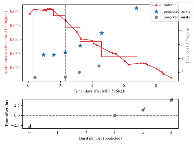
In the top panel, the accretion rate (red dots, left-hand y-axis) inferred from the persistent flux measurements are shown, joined by lines implying the use of linear interpolation (interp='linear') for flux inbetween. The measured fluence of the observed bursts are indicated (gray circles, right-hand y-axis) along with the predicted bursts (blue stars). The time of the reference burst is indicated (black dashed line). For the purposes of simulation the code assumes the accretion rate is constant between the predicted bursts, which is indicated by the stepped red line.

The lower panel shows the time offset between the predicted and observed bursts. In this example the times of the bursts are reproduced reasonably well (the second burst doesn’t count, as its our reference from which the simulation is performed in each direction). There are two intermediate simulated burst falling between the first and second observed bursts, but there is also a net trend in the residuals. So our overall burst rate is a little low (and the fluences are too high). Even so, the agreement might be good enough to use the chosen theta as a starting point.

Note that the lower panel will not be shown if it’s not possible to match the observed and predicted bursts (e.g. if there are not sufficient predicted bursts) or if you pass the option show_model=False to the beansp.Beans.plot() method.

Each of the initialisation parameters are described in more detail below:

• run_id A string identifier to label each code run you do. It can include the location that the chains and analysis are saved. E.g. if I were modelling SAX J1808.4–3658 I would choose something like run_id = "1808/test1". If the package is installed as recommended, you can run the code from within the directory in which you wish to store the output The run_id will also specify the name of the .ini file that will be saved as a record of the run parameters, and can be used to restart/redo the run by initialising a new beansp.Beans object via the config_file parameter

• obsname Path to observation data file. Should be a string, e.g. beans/data/1808_obs.txt. Set to None to trigger an “ensemble” run

• burstname (required) Path to burst data file. Should be a string, e.g. beans/data/1808_bursts.txt

• gtiname Path to GTI data file. Should be a string, e.g. beans/data/1808_gti.txt. Set to None (the default) to turn off GTI checking

• theta Sets the initial location of your walkers in parameter space.

• numburstssim In “burst train” mode, this is the number of bursts to simulate in each direction. I.e. set to roughly half the number of bursts you want to simulate, to cover your entire observed train. Don’t forget to account for missed bursts! In “burst ensemble” mode this is just the number of bursts, so set as equal to the number of bursts observed.

• bc Bolometric correction to apply to the persistent flux measurements, in “burst train” mode. If they are already bolometric estimates just set this to 1.0.

• interp Interpolation method to average the persistent flux between bursts; options are linear (the default) and spline. If the latter is chosen, you can also define the smoothing length with the smooth parameter (defaults to 0.02)

• ref_ind Index of the adopted reference burst, for “burst train” mode. In this mode the code simulates the burst train both forward and backward in time, so the reference burst should be in the middle of predicted burst train; don’t forget Python indexing starts at 0. This burst will not be simulated but will be used as a reference to predict the times of other bursts.

• test_model Set to False to skip the model test on init; default is True

• threads This is required because the MCMC chains are run in parallel, so you need to specify how many threads (or how many cores your computer has) that will be used.

• restart If your run is interrrupted and you would like to restart from the save file of a previous run with the run_id set above, set this to True. Can also be used if your max step number was not high enough and the chains did not converge before the run finished if you want to start where it finished last time. If this is a new run, set this to False.

• config_file Read in the parameters from the named file (.ini extension) rather than specifying by hand

Some additional parameters can be used to control the behaviour of the sampler:

• sampler The sampler you want to use. The default is emcee, but you can also use dynesty provided bilby is also installed

• nwalkers The number of walkers you want the emcee algorithm to use. Something around 200 should be fine. If you are having convergence issues try doubling the number of walkers - check out the emcee documentation for more information.

• nsteps The desired number of steps the emcee algorithm will take. Every 100 steps the code checks the autocorrelation time for convergence and will terminate the run if things are converged. So you can set nsteps to something quite large (maybe 10000), but if things are not converging the code will take a very long time to run.

• nlive The number of “live” points for the dynesty sampler.

• dlogz The convergence criterion for the dynesty sampler.

• prior Use the specified function in place of the default prior; an example which can be adapted to different sources is beansp.beans.prior_1808()

• corr Use the specified function to modify the results from pySettle; an example is beansp.beans.corr_goodwin19()

• alpha Set to False to ignore the alpha measurements in the likelihood; default is True

• fluen Set to False to ignore the fluen measurements in the likelihood; default is True

If there are no errors or other issues here, move on to running the code.

3. Running the Code

Once you have initialised the beansp.Beans object and ensured all the data is available, you are ready to go. Running the code is done with the following command:

B.do_run()

If all is well you will see a progress bar appear which will give you an idea of how long the run is going to take.

When you see Complete! Chains are converged this means the run finished, and the chains were converged.

When you see Complete! WARNING max number of steps reached but chains are not converged. This means the run finished but reached the maximum number of steps nsteps without converging.

Practically it’s useful to start with a few shorter runs to verify the operation, e.g. checking that the chains are evolving in a plausible direction (with the chain option below).

Once you have a preliminary run that you would like to continue, you can do so by setting restart=True in the beansp.Beans object. This will automatically continue from the last walker position, appending the new results to the existing .h5 file.

More fine-control of the walker positions is possible with the pos option to beansp.Beans.do_run():

B.do_run(pos=custom_positions)

This option will use the supplied array (dimension nwalkers x ndim) as the starting points.

Checking Chain Convergence

There are two main methods of checking the convergence and behaviour of your emcee chains. One is the autocorrelation time, which emcee conveniently calculates for you, and the other is the acceptance fraction. Goodman and Weare (2010) provide a good discussion on what these are and why they are important; see also the tutorial with emcee.

Running B.do_analysis(['autocor']) (see below) will display the integrated autocorrelation time and the estimates from emcee.

4. Analysing the Results

The output of the MCMC algorithm is saved in HDF5 format, and will be located in whichever folder you chose when you set run_id. For initial analysis of the chains you can run:

B.do_analysis()

And it will create a plot showing the estimated autocorrelation times throughout the run, as well as the posterior distributions of your parameters.

Typically you will omit the initial “burn-in” phase and only use the walker positions in the later part of the run; you can specify how many steps to skip with the burnin parameter.

The model predictions at each step are saved in the “blobs” part of the sampler, which are used together with the parameter values to display the various plots below. For compatibility with the HDF5 format the model prediction dictionary must be converted to a string, and so it needs to be turned back into a dictionary item-by-item (e.g. with eval) when you read in the save file.

Several other options are possible for built-in analysis, and can be specified via the options keyword to beansp.Beans.do_analysis(), which accepts a list of strings, specifying one or more of:

autocor

plot estimates of the autocorrelation times for each parameter, as a function of timestep

chain

plot the first 300 iterations of the chains

posteriors

show a “corner” plot giving the distirbution of the raw posteriors of the model parameters

mrcorner

show a “corner” plot with just the neutron star parameters, M, R, g and 1+z

fig6

replicate Figure 6 from Goodwin et al. (2019), a “corner” plot with xi_b, xi_p, d, Q_b, Z

fig8

replicate Figure 8 from Goodwin et al. (2019), plotting xi_b vs. xi_p and models (where available, via the concord repository) for comparison’,

comparison

plot the observed and predicted burst times and fluences

You can choose to display the figures for each analysis, or save to a PDF by specifying savefig=True in the call to beansp.Beans.do_analysis().

Observed-predicted burst time comparisons

The comparison analysis option behaves in a special way, which affects some of the other analyses. Depending on the range of walkers, you may have different numbers of predicted bursts at different walker positions. The comparison analysis will group these and plot their burst statistics separately, to help you gauge which is the best option to pursue (for example).

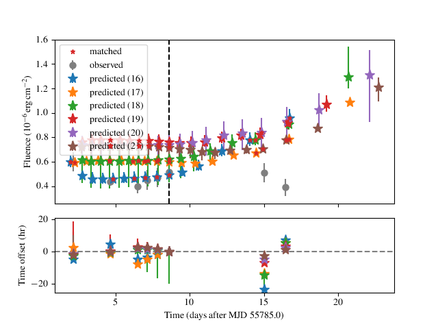
An extreme example is shown for a run for IGR J17498-2921 above, where there are 6 different solution sets with different numbers of predicted bursts. The relative agreement can be gauged in the residual plot in the lower panel, as well as the RMS offset between the predicted and observed bursts, which is displayed for each model. In this case the 21-burst solution is the preferred one, with an RMS error of only 1.92 hr.

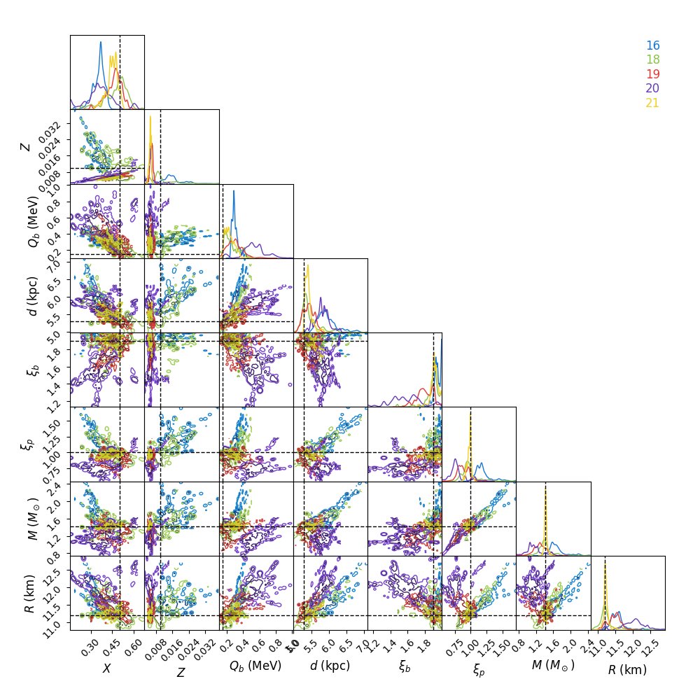
The different solutions corresponding to different burst numbers are retained in the posterior object, so that if you subsequently call the posteriors option in beansp.Beans.do_analysis() the posteriors will also be plotted separately for each different group. For the extreme case above the posteriors get rather busy…

To “home in” on the best solution you could recover the last set of samples and choose only those walkers fitting the 21-burst solution:

p, *dummy = B.reader.get_last_sample()
np.shape(p)
(200, 8)
good = np.array(B.model_pred['partition'])[-200:] == 21
len(np.where(good)[0])
39

Only 39 samples are not so many to continue with the run, but you could use them as a starting point and distribute new walkers around them, and continue the runs from these positions using the pos option to beansp.Beans.do_run() (see above).

Obtaining Parameter Constraints

The model parameter posterior distributions are the most detailed constraints on your parameters provided by the MCMC algorithm. However, you may wish to summarise by giving central values with uncertainties to report for the parameters. There are a few ways this can be done; e.g. take the maximum likelihood value and the upper and lower limits encompassing the desired confidence fraction, or you could take the 50th percentile value of the distributions. The analysis code in beansp.Beans.do_analysis() does this one way, but you should always check multiple methods and see if the results are significantly different.

Call beansp.Beans.write_param_uncert() to save the central values of these and 1 sigma uncertainties in the text file (run_id)_parameterconstraints_pred.txt.

The model predictions include the burst time, fluence, and alpha, which are stored as arrays containing an entry for each of the predicted bursts. These arrays will include as many elements as are chosen via the numburstssim parameter on initialisation. The time array has 1 extra element than the fluence and alpha arrays, because the latter parameters do not include predictions for the reference burst (with index ref_ind).